Stage I / Adapt
Targeted Truck-SFT
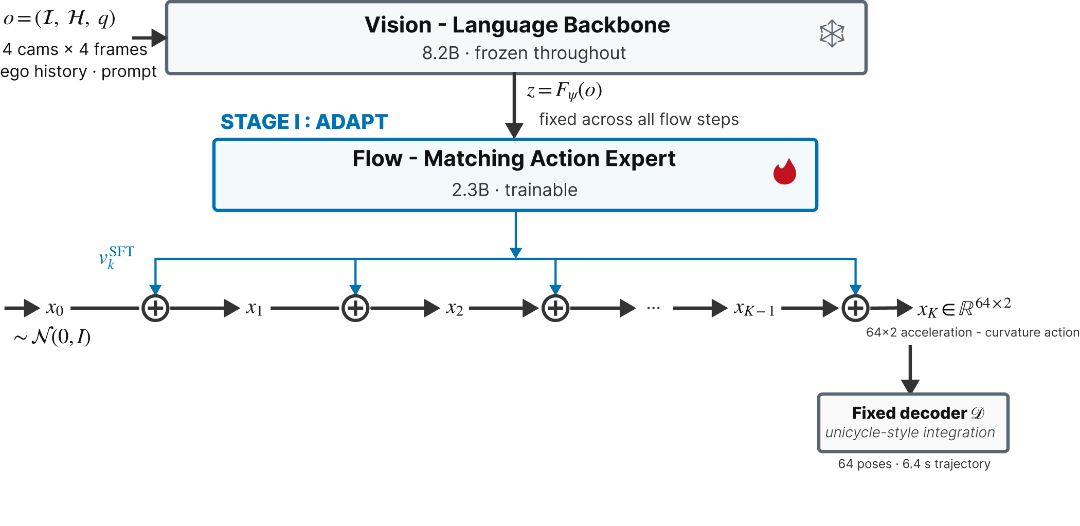
We fine-tune the action-generation stack on 229 targeted truck scenarios. The vision-language backbone stays frozen.
1 University of Southern California2 Stack AV


The paper link will be added with the arXiv release.
A code link is not available yet.
Adapted = Targeted SFT + FVS.
Accident I · Kcand = 1 · 6.4 s prediction horizon · Open-loop evaluation
Class 8 trucks differ from passenger cars in geometry, dynamics, and maneuvering requirements. We propose an adapt-then-steer strategy that uses limited targeted demonstrations to adapt vision-language-action (VLA) models for generating candidate trajectories in long-tail truck-driving scenarios. In the adapt stage, we use NVIDIA’s Alpamayo 1.5 as the base model, fine-tuning only its action-generation stack on a few hundred real-world construction and accident-related highway scenarios. In the steer stage, we introduce Flow Velocity Steering (FVS) to further refine the model’s predictions while holding the adapted VLA fixed. FVS is a compact, flow-time-conditioned residual module that adds learned corrections to the action-space flow velocity used to update the action sequence at each generation step. In open-loop evaluation on a scenario-disjoint held-out set, targeted fine-tuning more than halves single-candidate average displacement error (ADE) and final displacement error (FDE) over the entire 6.4 s horizon compared to the base model. Using the same targeted demonstrations, FVS further reduces the fine-tuned model’s full-horizon ADE and FDE by 13.9% and 16.5%, respectively. At matched data budgets, targeted supervision yields 19–26% lower full-horizon ADE than general truck-driving supervision, while the targeted model remains competitive with one fine-tuned on approximately 65× as many general truck-driving scenarios. These results support adapt-then-steer for data-efficient vehicle-domain transfer to Class 8 trucks.
01 / Motivation
We study how to adapt a driving VLA to Class 8 trucks, which differ from passenger cars in sensor viewpoint, articulated geometry, vehicle dynamics, and maneuvering requirements.
We study whether limited targeted demonstrations can adapt a pretrained driving VLA to better match expert truck trajectories in construction and accident-related highway scenarios, without retraining its vision-language backbone.
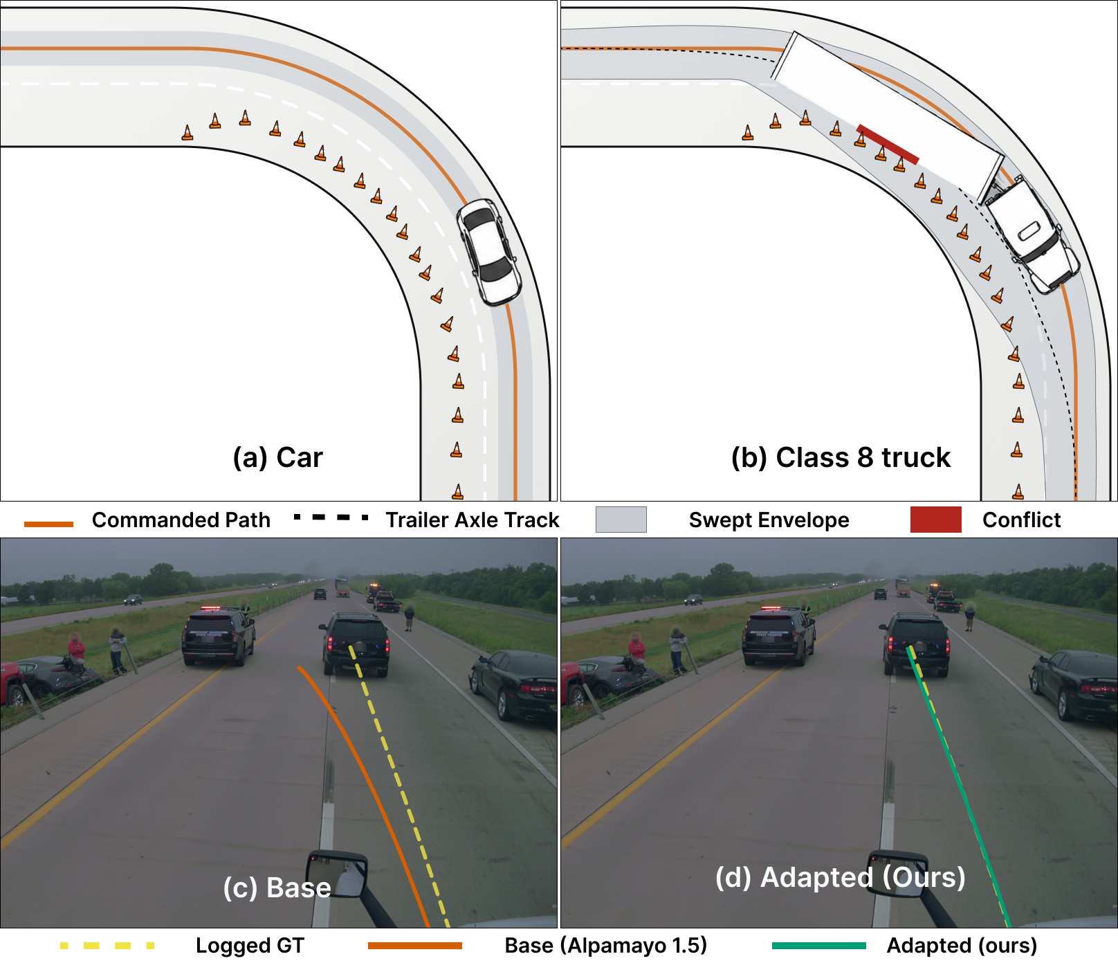
The figure illustrates one motivating geometric example: under the same reference path, a passenger car clears a work-zone closure, while trailer off-tracking carries an articulated truck’s swept envelope into it.
02 / Method
We first adapt the model using truck demonstrations. We then train FVS to refine its predictions while keeping the adapted model frozen.
We first adapt the action-generation stack, then refine it with FVS.
Step 1 of 2
In Stage 1, we fine-tune the model’s action-generation stack on 229 targeted truck scenarios while keeping the vision-language backbone frozen.
Step 2 of 2
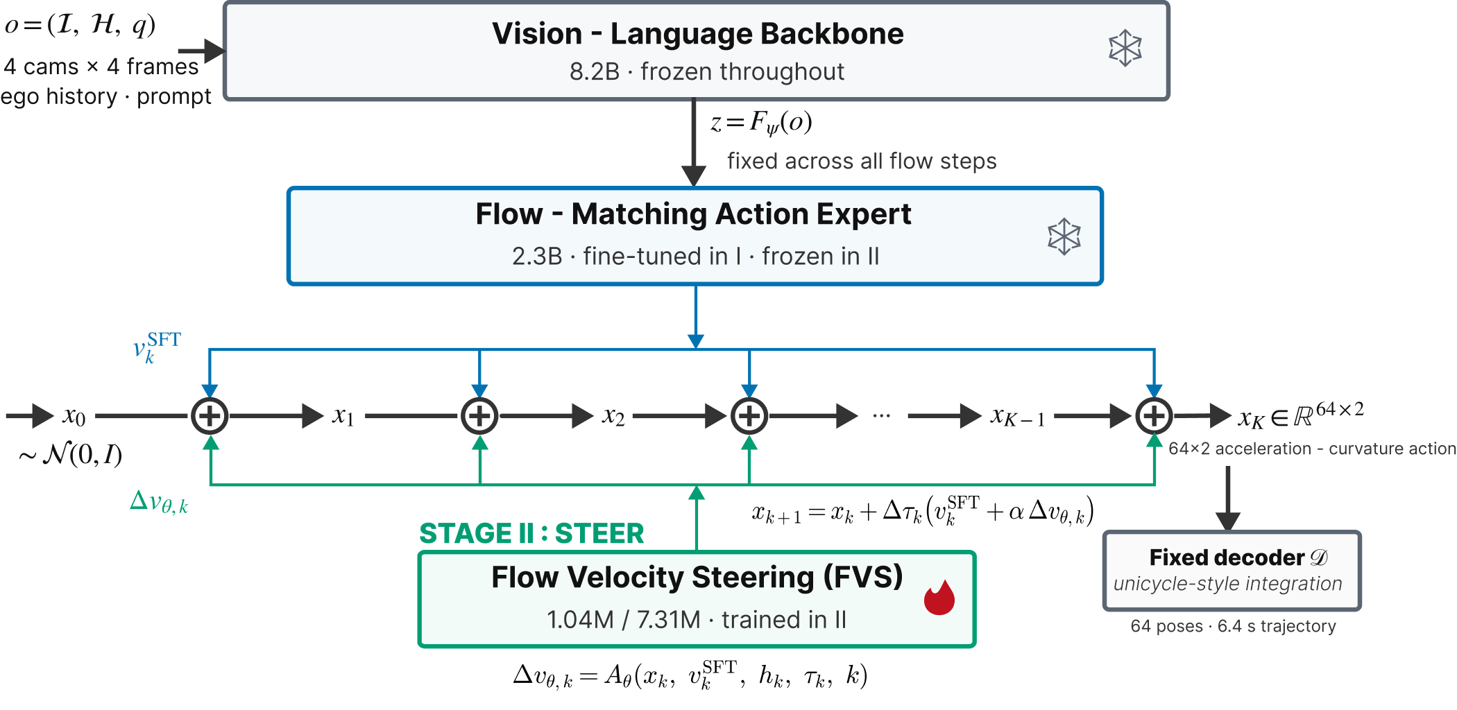
FVS is a compact, flow-time-conditioned residual module that corrects action-space flow velocity at each generation step. We train it on the same demonstrations while keeping the adapted model frozen.
Swipe across the diagram, or tap it to enlarge.
Stage I / Adapt
We fine-tune the action-generation stack on 229 targeted truck scenarios. The vision-language backbone stays frozen.
Stage II / Steer
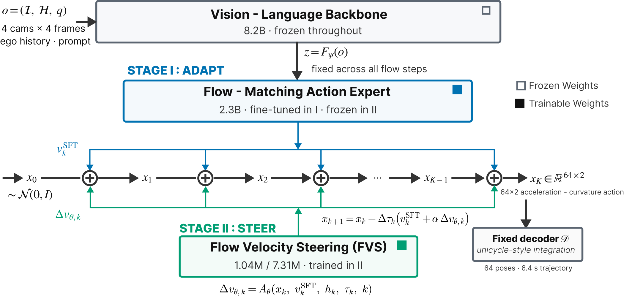
FVS is a compact, flow-time-conditioned residual module that corrects action-space flow velocity at each generation step. We train FVS on the same demonstrations while keeping the adapted model frozen. FVS adds 7.31M trainable parameters, less than 0.1% of the base model.
Steered Euler update in normalized action space
vkSFT is the frozen Action Expert’s nominal flow velocity, while Δvθ,k is the learned FVS correction.
 View full figure ↗
03 / Test scenarios
We compare Base, Targeted SFT, and FVS on four unseen test scenarios that were not used for Targeted SFT or FVS training. Each comparison uses the same observations, 6.4 s prediction horizon, and inference-noise seed.
4(a) · Accident-related
We compare Base (left) with FVS (right), both against GT. Adapted means Targeted SFT + FVS.We compare Base (top) with FVS (bottom), both against GT. Adapted means Targeted SFT + FVS.
We compare GT, Base, and Targeted SFT to show the effect of fine-tuning.We compare GT, Base, and Targeted SFT to show the effect of fine-tuning.
We compare SFT (left) with FVS (right). Both panels include GT and Base; FVS uses the same frozen SFT model.We compare SFT (top) with FVS (bottom). Both panels include GT and Base; FVS uses the same frozen SFT model.
We show all 16 candidates from Base, SFT, and FVS in separate panels, ordered left to right. Each panel includes the same GT trajectory. Shading shows candidate spread, not a physical truck swept envelope or confidence interval.We show all 16 candidates from Base, SFT, and FVS in separate panels, ordered top to bottom. Each panel includes the same GT trajectory. Shading shows candidate spread, not a physical truck swept envelope or confidence interval.
4(b) · Accident-related
We compare Base (left) with FVS (right), both against GT. Adapted means Targeted SFT + FVS.We compare Base (top) with FVS (bottom), both against GT. Adapted means Targeted SFT + FVS.
We compare GT, Base, and Targeted SFT to show the effect of fine-tuning.We compare GT, Base, and Targeted SFT to show the effect of fine-tuning.
We compare SFT (left) with FVS (right). Both panels include GT and Base; FVS uses the same frozen SFT model.We compare SFT (top) with FVS (bottom). Both panels include GT and Base; FVS uses the same frozen SFT model.
We show all 16 candidates from Base, SFT, and FVS in separate panels, ordered left to right. Each panel includes the same GT trajectory. Shading shows candidate spread, not a physical truck swept envelope or confidence interval.We show all 16 candidates from Base, SFT, and FVS in separate panels, ordered top to bottom. Each panel includes the same GT trajectory. Shading shows candidate spread, not a physical truck swept envelope or confidence interval.
4(c) · Construction
We compare Base (left) with FVS (right), both against GT. Adapted means Targeted SFT + FVS.We compare Base (top) with FVS (bottom), both against GT. Adapted means Targeted SFT + FVS.
We compare GT, Base, and Targeted SFT to show the effect of fine-tuning.We compare GT, Base, and Targeted SFT to show the effect of fine-tuning.
We compare SFT (left) with FVS (right). Both panels include GT and Base; FVS uses the same frozen SFT model.We compare SFT (top) with FVS (bottom). Both panels include GT and Base; FVS uses the same frozen SFT model.
We show all 16 candidates from Base, SFT, and FVS in separate panels, ordered left to right. Each panel includes the same GT trajectory. Shading shows candidate spread, not a physical truck swept envelope or confidence interval.We show all 16 candidates from Base, SFT, and FVS in separate panels, ordered top to bottom. Each panel includes the same GT trajectory. Shading shows candidate spread, not a physical truck swept envelope or confidence interval.
4(d) · Construction
We compare Base (left) with FVS (right), both against GT. Adapted means Targeted SFT + FVS.We compare Base (top) with FVS (bottom), both against GT. Adapted means Targeted SFT + FVS.
We compare GT, Base, and Targeted SFT to show the effect of fine-tuning.We compare GT, Base, and Targeted SFT to show the effect of fine-tuning.
We compare SFT (left) with FVS (right). Both panels include GT and Base; FVS uses the same frozen SFT model.We compare SFT (top) with FVS (bottom). Both panels include GT and Base; FVS uses the same frozen SFT model.
We show all 16 candidates from Base, SFT, and FVS in separate panels, ordered left to right. Each panel includes the same GT trajectory. Shading shows candidate spread, not a physical truck swept envelope or confidence interval.We show all 16 candidates from Base, SFT, and FVS in separate panels, ordered top to bottom. Each panel includes the same GT trajectory. Shading shows candidate spread, not a physical truck swept envelope or confidence interval.
04 / Quantitative results
| Method | ADE@6.4s ↓ | FDE@6.4s ↓ |
|---|---|---|
| Base | 2.6358 ± 0.1493 | 7.1830 ± 0.2868 |
| Targeted Truck-SFT | 1.1650 ± 0.0184 | 3.1590 ± 0.0213 |
| FVS (Transformer) | 1.0035 ± 0.0035 | 2.6383 ± 0.0156 |
SFT versus Base. We find that Targeted SFT reduces scenario-mean ADE@6.4s relative to Base in all 26 held-out test scenarios.
FVS versus SFT. We find that Transformer FVS further reduces scenario-mean ADE@6.4s relative to Targeted SFT in all 26 held-out test scenarios.
| Method | Kcand = 1 · Single candidate | Kcand = 16 · Oracle best-of-16 | ||||||
|---|---|---|---|---|---|---|---|---|
| ADE@1s | ADE@3s | ADE@6.4s | FDE@6.4s | minADE@1s | minADE@3s | minADE@6.4s | minFDE@6.4s | |
| CTRV | 0.1643 | 0.7003 | 2.0430 | 5.8412 | N/A | N/A | N/A | N/A |
| Base | 0.1530 ± 0.0018 | 0.6836 ± 0.0440 | 2.6358 ± 0.1493 | 7.1830 ± 0.2868 | 0.0621 ± 0.0001 | 0.2556 ± 0.0082 | 0.9402 ± 0.0038 | 2.3849 ± 0.0118 |
| Targeted Truck-SFT | 0.0600 ± 0.0008 | 0.3120 ± 0.0081 | 1.1650 ± 0.0184 | 3.1590 ± 0.0213 | 0.0413 ± 0.0004 | 0.1855 ± 0.0029 | 0.6968 ± 0.0115 | 1.8118 ± 0.0398 |
| General Truck-SFT | 0.0584 ± 0.0017 | 0.3146 ± 0.0194 | 1.2868 ± 0.0049 | 3.7404 ± 0.0824 | 0.0361 ± 0.0001 | 0.1659 ± 0.0051 | 0.6634 ± 0.0044 | 1.7652 ± 0.0240 |
| General → Targeted SFT | 0.0580 ± 0.0017 | 0.3121 ± 0.0168 | 1.2539 ± 0.0422 | 3.6012 ± 0.0703 | 0.0371 ± 0.0008 | 0.1716 ± 0.0045 | 0.6697 ± 0.0009 | 1.7587 ± 0.0313 |
| Final-Action Residual (MLP) | 0.0595 ± 0.0006 | 0.3060 ± 0.0043 | 1.1362 ± 0.0092 | 3.1071 ± 0.0186 | 0.0402 ± 0.0003 | 0.1813 ± 0.0012 | 0.6918 ± 0.0073 | 1.8001 ± 0.0232 |
| Final-Action Residual (Transformer) | 0.0589 ± 0.0006 | 0.3010 ± 0.0032 | 1.1276 ± 0.0081 | 3.0002 ± 0.0175 | 0.0391 ± 0.0003 | 0.1801 ± 0.0016 | 0.6876 ± 0.0051 | 1.7992 ± 0.0210 |
| FVS (MLP) | 0.0481 ± 0.0003 | 0.2659 ± 0.0004 | 1.0065 ± 0.0035 | 2.6527 ± 0.0171 | 0.0363 ± 0.0000 | 0.1658 ± 0.0001 | 0.6613 ± 0.0027 | 1.7419 ± 0.0115 |
| FVS (Transformer) | 0.0468 ± 0.0003 | 0.2656 ± 0.0009 | 1.0035 ± 0.0035 | 2.6383 ± 0.0156 | 0.0354 ± 0.0000 | 0.1642 ± 0.0006 | 0.6573 ± 0.0012 | 1.7003 ± 0.0102 |
ADE averages Euclidean position error through each horizon; FDE measures error at its endpoint. For Kcand = 16, each metric independently selects its lowest-error candidate before averaging across windows. This oracle best-of-set measure does not assume an online selector with access to GT. CTRV is deterministic; learned-model uncertainty reflects inference-noise variability for fixed checkpoints.
| Method | Lateral ADE (m) | Longitudinal ADE (m) | Heading error (°) |
|---|---|---|---|
| CTRV | 0.7958 | 1.6934 | 1.6162 |
| Base | 1.0204 ± 0.0638 | 2.1706 ± 0.2306 | 3.2926 ± 0.8549 |
| Targeted Truck-SFT | 0.4749 ± 0.0130 | 0.9323 ± 0.0197 | 0.8851 ± 0.0232 |
| General Truck-SFT | 0.4832 ± 0.0152 | 1.0929 ± 0.0402 | 1.1377 ± 0.0459 |
| General → Targeted SFT | 0.4932 ± 0.0140 | 1.0385 ± 0.0298 | 1.1192 ± 0.0553 |
| Final-Action Residual (MLP) | 0.4634 ± 0.0070 | 0.9115 ± 0.0115 | 0.8590 ± 0.0172 |
| Final-Action Residual (Transformer) | 0.4592 ± 0.0068 | 0.9009 ± 0.0117 | 0.8512 ± 0.0171 |
| FVS (MLP) | 0.4059 ± 0.0053 | 0.7738 ± 0.0127 | 0.7644 ± 0.0120 |
| FVS (Transformer) | 0.3870 ± 0.0051 | 0.7650 ± 0.0110 | 0.7169 ± 0.0105 |
Lateral and longitudinal ADE measure mean absolute VCP-position error along the corresponding axes. Final heading error is the absolute angular difference at 6.4 s. Values are mean ± sample standard deviation across inference-noise seeds, except deterministic CTRV.
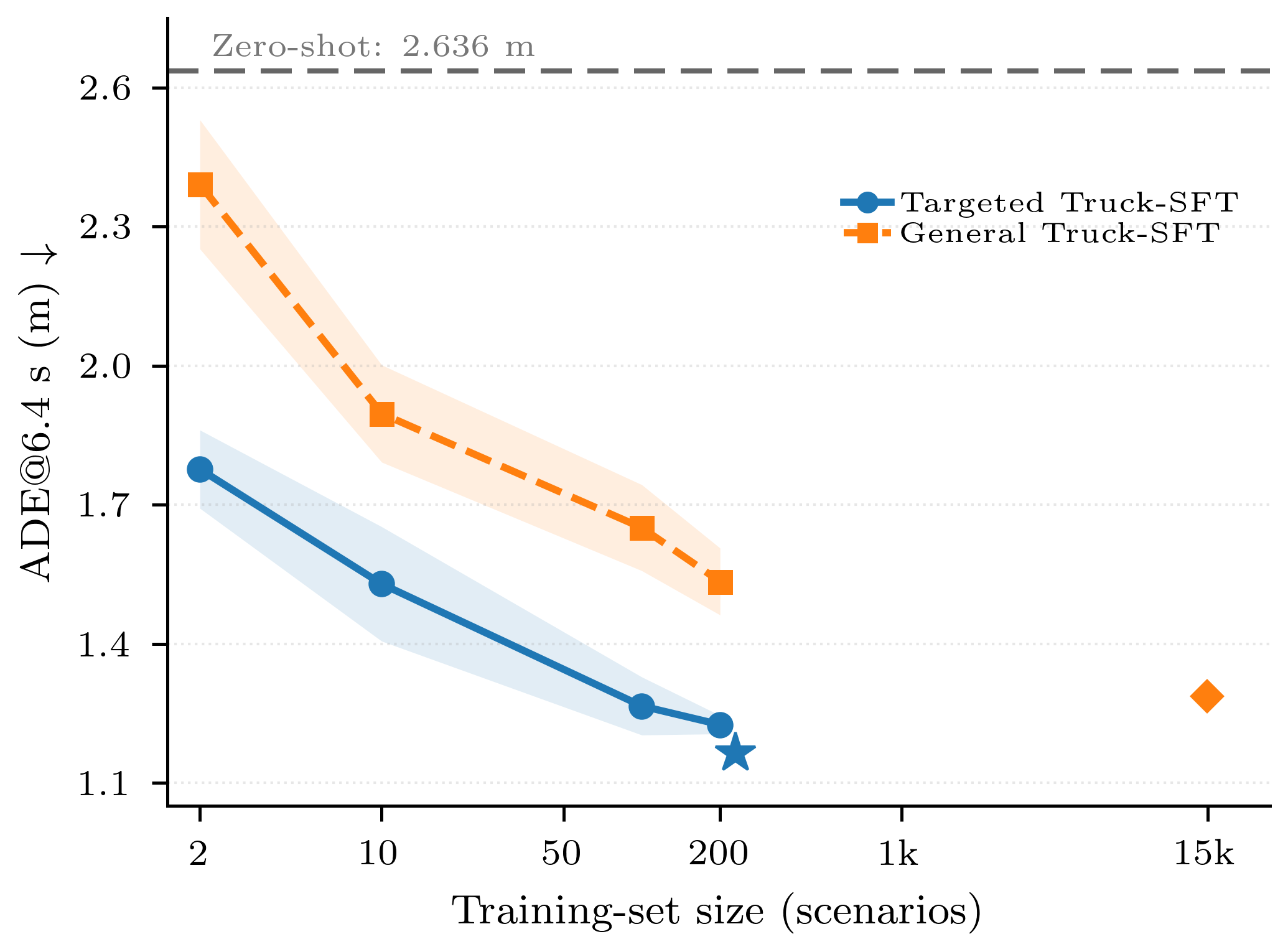
We compare targeted and general truck-driving supervision at matched training budgets of 2, 10, 100, and 200 scenarios. Targeted supervision yields 19–26% lower full-horizon ADE.
With 229 targeted scenarios, we obtain competitive trajectory accuracy compared with a model fine-tuned on 14,891 general truck-driving scenarios, approximately 65× as much data.
The ordering depends on the metric: general supervision performs better on some oracle best-of-16 measures. Sweep curves summarize three independently trained subset runs; full-data checkpoints are separate references.
 View full figure ↗
 View full figure ↗
05 / Reference
Citation to be updated.
% Citation details to be updated.
@misc{citation_to_be_updated,
  title = {To be updated},
  author = {To be updated}
}